Sign up here to receive Bellingcat’s biggest investigations by email as soon as they are published. Become a member and support our work here.

Imagery captured by the European Space Agency’s freely available Sentinel-2 and Sentinel-1 satellites appears to be delayed over Gaza and parts of the West Bank, a Bellingcat analysis has found.

While the delay remains relatively short at just 24 hours, this can still impact the speed at which analysts and researchers can observe what is happening in the region.

For example, the Israeli Defence Forces demolished homes in the West Bank Palestinian city of Hebron in recent days. New imagery captured on October 26, which included Hebron, would allow open source researchers to quickly confirm the demolitions, assess the impacted area and observe any unreported IDF activity. But imagery for the western half of Hebron was not available until October 27 due to the Sentinel-2 delay, inhibiting real-time fact-checking and reporting on this evolving situation.

A spokesperson for the European Union told Bellingcat that the delay was not related to events in Gaza but to “mitigate possible threats” due to the war in the Middle East “including Iran’s attacks on its neighbours and possible threats to European interests”. The delayed region of Sentinel tiles that cover Gaza as well as parts of Israel and the West Bank also extends over the Eastern Mediterranean Sea.

The European Union ordered a 24-hour delay on Sentinel satellite imagery over the Gulf of Oman earlier this year during US and Israeli strikes on Iran. However the delay impacting Gaza and parts of the West Bank has not been announced or previously reported.

“Such decisions are taken unanimously by all EU Member states and will stay in place as long as necessary,” the spokesperson said. They also said that while the Copernicus program, which includes the Sentinel satellites, operated a free and open data policy there were limitations to this for security. 

When asked if the delay, which began in late March, was related to the presence of US vessels in the Eastern Mediterranean or if there were other areas of delay, the spokesperson said they had no further comment.

Sentinel Delays

The Sentinel-2 and Sentinel-1 satellites provide an invaluable source of imagery for open source researchers. This has been especially true this year, as commercial satellite imagery providers restricted access to imagery in the Middle East, including areas of active human rights concern, such as Gaza. 

However, in July, the European Union published Council Decision 2026/1716, which ordered a 24-hour delay on Sentinel imagery over the Gulf of Oman, after a request from the US government which was involved in strikes on Iran at that time.

Just two weeks later, the European Union issued a corrigendum that unpublished decision 2026/1716 and removed it from the Council of the European Union record, although satellite data shows the delay has remained. 

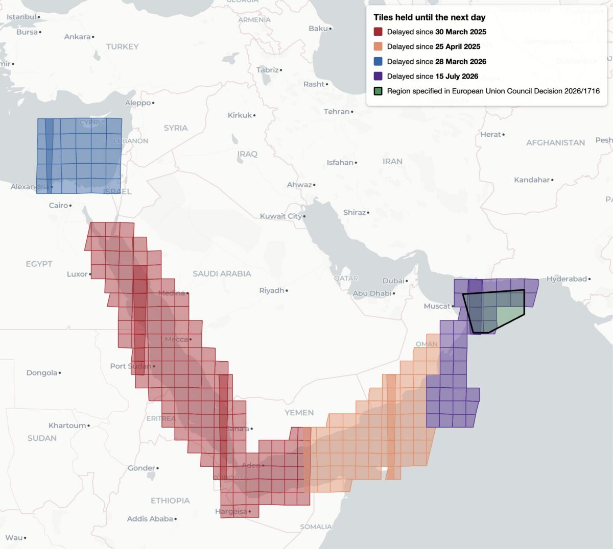
This decision, while it was available, was reportedly the first public notification of delayed Sentinel imagery. Yet it was not the first time that Sentinel imagery has been restricted, analysis shows. Bellingcat found four distinct regions of delayed satellite imagery during 2025 and 2026: the Gulf of Oman, the Gulf of Aden/western Arabian Sea, the Red Sea as well as the previously unreported delay in the Eastern Mediterranean Sea and parts of Israel, the West Bank and the entirety of Gaza.

Bellingcat’s analysis shows that these delays have been implemented in stages. Twenty-four hour delays of Sentinel-2 imagery were first observed by open source researchers in March and April 2025 after the US launched a naval and air strike campaign against Houthi targets in Yemen. 

The previously unreported imagery delay in the Eastern Mediterranean began on March 28, 2026, the same month that commercial American space imaging company Planet Labs also restricted imagery across the Middle East. The Gulf of Oman delay began on July 15, 2026, two days after the publication of Council Decision 2026/1716.

Decision 2026/1716 also specified that the delay be implemented for both Sentinel-2 and Sentinel-1 radar imagery. Bellingcat’s analysis of Sentinel-1 image availability shows that this is the case for both the Gulf of Oman region and the unreported region over the Eastern Mediterranean Sea. However, the 2025 restrictions on Sentinel-2 imagery in the Red Sea and Gulf of Aden are not implemented in Sentinel-1. 

Sentinel-1 imagery uses “synthetic aperture radar” to capture lower resolution radar images that can collect data at night and on cloudy days. This differs from Sentinel-2, which captures optical satellite imagery at higher resolution.

A Tale of Two Tiles

Sentinel satellite imagery is most commonly accessed by open source researchers through Copernicus Browser, a free online platform, but it is also distributed as large tiled files in the Copernicus Data Space Ecosystem. These tiles are numbered using the Military Grid Reference System, and can be listed using APIs that provide information on each tile, including the capture and publication time. By comparing the capture and publication time, the publication delay can be computed.

For example, the catalog information for the tile T36RXV, which includes Gaza and portions of the West Bank, Negev and Egypt, provides the following metadata for the October 21, 2026 capture.

This shows that while the image was captured at 08:20 UTC on October 21, it was not published until 10:09 UTC on October 22 — almost 26 hours later. This is in contrast to the neighboring tile T36RYV, which includes parts of the West Bank, Israel, and Jordan. API data for this tile shows that the image was published at 12:10 UTC on October 21, just under four hours after the capture time.

This difference is not unique to this date either. Bellingcat’s analysis shows that this tile has been consistently delayed by one day since March 28, 2026.

This method can be extended further, and by analysing every tile with valid publication date timestamps, Bellingcat identified all global Sentinel-2 and Sentinel-1 delays since 2023. The only consistent delays visible were those identified in the Gulf of Oman, the Gulf of Aden/western Arabian Sea, the Red Sea and Eastern Mediterranean in 2025 and 2026.

Impact on open source investigations

While the 24-hour delay on certain Sentinel imagery is a less severe restriction than other satellite providers have imposed, it can still impact the open source research process in fast moving situations. This is especially so in recent months as the European Space Agency’s Sentinel satellite data has emerged as a refuge as other satellite data is censored.

The image below shows how imagery for the eastern half of Hebron was visible on October 26, but not the western half where demolitions took place earlier this week.

The shape of the missing tiles can be seen by zooming out within the Copernicus browser, demonstrating how imagery of Gaza and other parts of Israel and the West Bank are also delayed.

Sentinel imagery covering western Hebron after the demolitions took place was published on October 27. However, the delay prevented local reports from being verified with satellite imagery while the situation was still ongoing.

Some Sentinel-2 users have previously described the challenges of covering fast-moving issues in the Gulf of Oman when the Sentinel delay was announced in March.

---

Bellingcat is a non-profit and the ability to carry out our work is dependent on the kind support of individual donors. If you would like to support our work, you can do so here. You can also subscribe to our Newsletter and follow us on Bluesky here, Instagram here, Reddit here and YouTube here.

The post EU Satellite Imagery Delayed Over Gaza and Parts of West Bank by 24-hours appeared first on bellingcat.

If you’ve seen reports of a wildfire in your region and you’re looking for open source data, NASA’s fire-tracking tool is often the first place to start. It provides a heat signature and an approximate location. But detection is only the first step in understanding what’s happened. In this guide, we explore ways to analyse and report on the scale and severity of wildfires, including those in protected areas where ecosystems are often most fragile. We also examine how often fires recur in the same region over multiple seasons, helping to identify patterns in fire activity as climate change reshapes fire risk around the world. 

Satellite imagery from Copernicus Browser will be used to visualise the spread of the fire, and vegetation health indices to assess burn severity. The datasets will then be combined in QGIS for more in-depth analysis. At each stage, suggestions will be offered for turning the data into clear, reportable findings.

Throughout this guide, a single case study will be used: Sicily’s Zingaro Nature Reserve. In 2025, wildfires swept across the region, destroying forests, grasslands and croplands. Located on the Capo San Vito peninsula, the reserve was so severely affected that sections remain closed today. 

Visualising Scorched Earth

When investigating a wildfire, it’s important to narrow down when it occurred and where it spread. The Landsat and Sentinel-2 missions are well-suited to this task, providing regular free imagery of most of the Earth’s landmass.

Below are two sets of Sentinel-2 imagery showing conditions shortly before and after a fire on July 25, 2025, near Capo San Vito, Sicily. The top two images are true-colour, similar to what would be seen from an aeroplane window. The image on the top right shows an area of scorched earth on the eastern side of the peninsula, but the exact extent of the fire is difficult to determine because the colour of the ground has changed only slightly.

The bottom two images are false-colour and highlight the difference between healthy vegetation and burned areas. Such imagery is possible because Sentinel-2 captures bands of light outside the visible range, a technique known as multispectral imaging. In these images, the near-infrared (NIR) band is coloured green, and the shortwave infrared (SWIR) band is coloured red. Healthy vegetation mainly reflects NIR light, so it appears green, while burned areas mainly reflect SWIR light, so they appear red.

These images were created with Copernicus Browser, a free browser-based tool from the European Space Agency for accessing and working with Sentinel imagery. It allows users to browse the Sentinel-2 catalogue by date and visualise different band combinations. You don’t need an account to use the browser, but signing in enables additional features.

If you’d like to try Copernicus Browser without further explanation, you can go straight to the false-colour post-fire image here. 

To follow along step by step, first open Copernicus Browser. Then to visualise Sentinel-2 imagery:

1. Zoom to the desired area on the map or use the search bar (San Vito Lo Capo, north-west Sicily)
2. Select the date of interest (‘2025-07-27’ selected below).
3. Select the layer of interest (‘True color’ by default; SWIR selected below).

By identifying the last available image before the fire and the earliest image after it in which the full burn area is visible, it’s possible to establish the location and timeline of the fire.

This allows us to report the following finding: “Satellite imagery reveals the extent of the damage caused by wildfires across the Capo San Vito peninsula on Sicily’s northern coast between July 20 and July 27, 2025.”

Extra exercise: Look up a recent fire (e.g., wildfires near Penco, Chile in January 2026), navigate to the affected location and try to visualise the burned area using Copernicus Browser.

Quantifying the Burned Area

The visibly scorched area can be measured using the Area of Interest tool (highlighted below), which allows users to draw a polygon on the map and calculate the total area in square kilometres. (Once drawn, keep the polygon in the editor, as it will be used again later.)

Reportable finding: “The wildfire that swept across Sicily’s Capo San Vito peninsula in 2025 burned more than 50 km2 of the peninsula, according to Sentinel-2 data.”

Repeatedly measuring the burned area over time allows you to follow the progression of a fire. This method was used by Bellingcat when covering the Etosha National Park wildfire in late September 2025.

Extra exercise: Replicate the analysis of the Etosha National Park fire from this Bellingcat article.

Assessing Burn Severity 

Some fires only affect surface vegetation, while others scorch the ground and cause long-lasting damage. Burn severity can be measured using an index called the Normalised Burn Ratio (NBR).

How Does the Normalised Burn Ratio (NBR) Detect Burned Areas?

The spectral response of a material describes how reflective it is to different types of light. The graph below shows the difference between healthy vegetation and bare soil in terms of the amount and types of light they reflect.

By focusing on the NIR and SWIR bands, where reflectivity differs significantly between healthy vegetation and bare soil left after a burn, an index can be calculated: 

NBR = (NIR – SWIR) / (NIR + SWIR) 

A high NBR indicates healthy vegetation, while a low NBR indicates burned areas.

Copernicus Browser doesn’t include a default NBR layer, but it can be added via a custom script, as shown in the screenshot below:

1. Select ‘Custom’ in the layer selector.
2. Switch from the ‘Composite’ to the ‘Custom’ tab.
3. Check ‘Load script from URL’.
4. Paste this URL: https://bellingcat-scripts.ams3.cdn.digitaloceanspaces.com/NormalizedBurnRatio.js 
5. Load the script by clicking the green circular arrows to the right of the URL.
6. Click ‘Apply’ (you may need to scroll down).

Alternatively, you can skip these steps and go straight to the custom NBR post-fire image here.

The NBR layer displays positive values in green (healthy vegetation) and negative values in purple (burned areas), making the boundary of the scorched area much clearer than before.

To calculate the change in NBR in Copernicus Browser, use the Statistical Information tool (a free account is required to access this feature).

1. Within the date selector, choose a date a few weeks or months after the fire.
2. Using the Area of Interest polygon, select the ‘Statistical Info chart’ icon.
   
   
   

3. Set the maximum cloud cover to around 30% using the slider in the top right.
4. Select a date range that captures the available data surrounding the fire (July 20-27 shown below).
5. Identify when the fire occurred on the graph (this will be marked by a sharp drop in the NBR, as shown below).
6. Hover over the points on the graph immediately before and after the fire to display the mean value.

In this example, the pre-fire image had an average NBR of 0.11 and the post-fire image had an average NBR of -0.18. The NBR decreased by 0.29, which represents a moderate burn.

Severity Level	Change in NBR
Unburned	Less than 0.100
Low	0.100 – 0.269
Moderate	0.270 – 0.659
High	0.660 or greater

Reportable finding: In late July, the fire, which scorched more than 50km2 of Sicily’s Capo San Vito peninsula, was deemed moderately severe according to the US Forest Service guidelines. 

Extra exercise: Find a custom visualisation script of interest from this repository and explore what it does.

Wildfires in Conservation Areas

By focusing on protected sites such as nature reserves and national parks, we can begin to assess how wildfires affect areas of high conservation value. Controlled burns are widely used in agriculture and land management, but unchecked fires in protected areas risk eroding fragile ecosystems.

The proportion of the Zingaro Nature Reserve that was damaged by the fire can be estimated by combining the NBR image created in Copernicus Browser with a dataset from Protected Planet, a global map of protected areas that includes nature reserves.

QGIS, a program for working with geographic data, is well-suited for this type of analysis. Download and install QGIS on your computer. For help with this step, refer to the QGIS installation guide.

To download the NBR image from Copernicus Browser:

1. With the NBR visualisation selected, click the ‘Download’ icon. 
2. Switch tabs at the top from ‘Basic’ to ‘Analytical’.
3. Change the image format to ‘TIFF (32-bit float)’.
4. Change the image resolution to ‘HIGH’.
5. Change the coordinate system to ‘Popular Web Mercator (EPSG:3857)’.
6. Toggle the ‘Clip extra bands’ switch to the off position (see image below).
7. Select the ‘Custom’ layer check box (and deselect any others).
8. Click ‘Download’.
9. Wait. It could take several minutes for the image to be generated and downloaded.

Once the image has downloaded, rename it to NBR.tiff to make it easier to work with. 

Next, open QGIS and click ‘New Project’ in the upper left. 

Load the image from Copernicus Browser by dragging and dropping the downloaded file into QGIS.

Useful QGIS Terminology

CRS – The Coordinate Reference System describes how the world should be measured and projected. Two of the most common are:

EPSG:4326 – WGS 84, which uses latitude and longitude as the unit of measurement.

EPSG:3857 – WGS 84 / Pseudo-Mercator, which uses metres as the unit of measurement.

Raster – a type of data that uses pixels to represent information (such as satellite imagery)

Vector – a type of data that uses points, lines, and polygons to represent information (such as a burn area polygon).

Processing the NBR Image

Next, we categorise each pixel in the NBR image as burned or unburned. 

Previous analysis in Copernicus Browser showed that the Zingaro Nature Reserve’s NBR value dropped below zero only after the fire (before image: mean NBR value on July 20, 0.11; after image: mean NBR value on July 27, -0.18).

We can use this analysis to set a threshold; anything below zero will be categorised as burned.

The QGIS Raster Calculator lets us apply our threshold to the NBR image and create a new layer. 

Open the Raster Calculator by selecting ‘Raster > Raster Calculator…’ from the menu bar at the top.

The Raster Calculator lists the raster bands available in the project. In this example, there are five. These bands are set by the custom script we used in Copernicus Browser and are numbered as follows:

1. Red
2. Green
3. Blue
4. Pixel validity (not used in this example)
5. NBR index

To create a new raster layer that applies our threshold on the NBR index band:

1. Double-click the fifth band (ending ‘@5’) to add it to the expression box at the bottom. 
2. Add < 0 using your keyboard (shown above).
3. Select the ‘Create on-the-fly raster instead of writing layer to disk’ checkbox.
4. Click ‘OK’.

The expression NBR@5 < 0 tells QGIS to categorise NBR index values as burned if they are less than zero. 

The new layer shows burned areas as white (a value of 1), and unburned areas as black (a value of 0).

Extra exercise: Download an NBR image captured before the fire. Use the Raster Calculator to create a new layer that shows burn severity.

Adding Conservation Area Data

Download the Zingaro Nature Reserve dataset from Protected Planet by selecting ‘Download > File Geodatabase’.

As before, drag and drop the downloaded file into QGIS. This time, the download is a zip file and contains many PDF files as well as the geodatabase file of interest. Scroll down to the bottom of the list and select the ‘gdbtable’ file with a polygon icon on the left side (see the blue highlighted row below), then press ‘Add Layers’.

This adds the nature reserve polygon as a layer in QGIS (and gives it an arbitrary colour). The nature reserve is almost completely contained within the white burned area, indicating it was heavily affected by the wildfire.

Quantifying the Burned Area in the Nature Reserve

To measure the proportion of the nature reserve that was burned by the wildfire, we will use the Zonal Histogram tool from the QGIS Processing Toolbox to count the number of unburned and burned pixels within the reserve polygon.

Open the toolbox with ‘Processing > Toolbox’, and a pane should open to the right. In the Processing Toolbox search field, look up ‘Zonal Histogram’ and double-click the result to open the tool.

To create a new layer:

1. Set the ‘Raster layer’ to the threshold burn area layer (NBR@5 < 0)
2. Set the ‘Vector layer containing zones’ to the nature reserve polygon layer (should start with ‘WDPA_’).
3. Click ‘Run’
4. Click ‘Close’

This will create a new layer called ‘Output zones’, which is a copy of the nature reserve polygon with pixel counts added.

Select the output layer in the lower left and click ‘Attribute Table’ in the upper right. (The attribute table is a spreadsheet-like view of the data contained in a layer.) 

For the output layer, there is just one row because there is only one polygon. If the layer contained many polygons, there would be many rows.

The newly calculated counts are added to the end of the table, so scroll all the way to the right. Look for fields starting with ‘HISTO_’. Here, HISTO_0 is the count of unburned pixels (value of 0), and HISTO_1 is the count of burned pixels (value of 1).

To calculate the proportion of burned area, the number of burned pixels is divided by the total number of pixels.

Proportion = 57413 / (57413 + 2195) = 0.96318…

A value of 0.96318 means that just over 96.3% of the nature reserve burned.

Reportable finding: In late July, more than 95% of the Zingaro Nature Reserve burned in a wildfire, according to Sentinel-2 satellite imagery and Protected Planet data.

Tracking Past Wildfires

To assess the significance of an ongoing wildfire, it is important to place it in historical context. How does it compare with previous fires in the same area? Is it part of a seasonal pattern, or does it represent an unusually severe event?

With coverage dating back to 2008, the European Forest Fire Information System (EFFIS) automatically maps wildfires across Europe, North Africa, and parts of the Middle East.

Fire data can be requested directly from EFFIS using web form, with results delivered by email. For ease, you can also download Bellingcat’s archived copy of EFFIS wildfire data for Italy covering 2015–2025.

For this section, it is best to open a new QGIS project.

To view and analyse historic wildfires in the Zingaro Nature Reserve using EFFIS data:

1. (Optional) Add the OpenStreetMap layer from the XYZ Tiles category by double-clicking it.
2. Load the EFFIS data into QGIS. If prompted to select a coordinate transformation, click ‘OK’ to accept the default option. 
3. Load the Protected Planet Zingaro Nature Reserve polygon as described earlier. 
4. Open the Vector Intersection tool by selecting ‘Vector > Geoprocessing Tools > Intersection…’ from the menu bar at the top.

The Intersection tool creates a new layer containing only the fires that affected the Zingaro Nature Reserve. To create the new layer:

5. Set the ‘Input layer’ to the EFFIS fires layer.
6. Set the ‘Overlay layer’ to the Zingaro Nature Reserve polygon layer.
7. Click ‘Run’.

QGIS functionality can be extended through plugins, including Data Plotly, which adds data visualisation tools. To install Data Plotly, open the Plugin Manager by selecting ‘Plugins > Manage and Install Plugins…’ from the menu bar, then:

8. Search for ‘Data Plotly’ in the available list.
9. Select the plugin from the search results.
10. Click ‘Install Plugin’ to download and install it. 

Once installed, open the Data Plotly panel with ‘View > Panels > DataPlotly’. The panel should appear on the right-hand side of the QGIS window. 

To plot a graph of historic wildfire activity within the nature reserve, configure Data Plotly as follows:

1. For ‘Plot type’, choose ‘Bar Plot’.
2. Set the ‘Layer’ to the newly created ‘Intersection’ layer.
3. In ‘X field’, type “year(initialdat)”. This expression extracts the year from the fire’s approximate start date, allowing events from the same year to be grouped together. 
4. In ‘Y field’ enter “$area/1000000”. This expression calculates the burned area within the nature reserve in square kilometres.

Note: EFFIS data provide initial and final dates for each fire, which are approximate because they depend on the availability of satellite imagery. These dates should be treated as bounds for when a fire occurred, rather than as the dates when it started and ended.

Next, switch to the Layout tab in Data Plotly:

5. Untick ‘Show Legend’. Only do this for simple plots where a legend is not required. 
6. Add a title and labels for the X and Y axes.
7. Finally, click ‘Create Plot’ and wait a few seconds for the chart to be generated.

The chart shows that the Zingaro Nature Reserve has experienced several significant wildfires over time. However, in 2025, the data show that the fire burned a larger area within the reserve than the major fires recorded in 2020 and 2017.

Reportable finding: The Zingaro Nature Reserve has experienced three major wildfires since 2015. Of these, the 2025 fire burned a larger area within the reserve than those recorded in 2020 and 2017.

The tools and methods in this guide can be applied to wildfires in many other regions. By combining satellite imagery with environmental and historical datasets, it’s possible to move beyond detection and begin to quantify a fire’s impact. In doing so, you can also place individual incidents in context, revealing whether they are part of a recurring pattern or an unusually severe event.

To learn more about fire detection, see Bellingcat’s guide to NASA FIRMS.

To explore QGIS further, visit the Bellingcat toolkit entry on QGIS.

---

Merel Zoet and Claire Press contributed to this report.

This guide contains modified Copernicus Sentinel data (2025), processed with Copernicus Browser, as well as data from the European Forest Fire Information System (EFFIS) of the European Commission Joint Research Centre.

Bellingcat is a non-profit and the ability to carry out our work is dependent on the kind support of individual donors. If you would like to support our work, you can do so here. You can also subscribe to our Patreon channel here. Subscribe to our Newsletter and follow us on Bluesky here, Instagram here, Reddit here and YouTube here.

The post Burning Forests: Tools for Tracking and Reporting Wildfire Damage appeared first on bellingcat.